C1 Rice
C1.1 Introduction
-
Capacities taught in this chapter
Reading and interpretingHow has rice consumption changed over the course of Indian history?Scientific processHow has rice evolved?Scientific toolsHow can we classify rice varieties?
How do we represent the evolutionary relationships among rice varieties?Bridging science, society and the environmentWas rice always part of our diet?
Has increased rice consumption caused undesirable health outcomes?Quantitative skillsHow do we represent the association between two variables?
- Holocene period
- The current geological epoch with significant human impact, that started approximately 11 700 years before the present. See also: epoch.
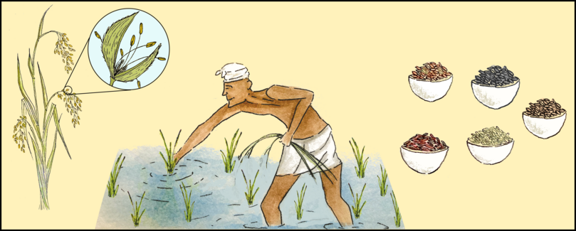
Early humans lived as hunter-gathering societies, subsisting on wild animals and plants. Later, societies evolved that practised agriculture and the domestication of crops. The domestication of staple cereals or crops tracks the major ecological, economic, political, and cultural transitions that occurred during the Holocene period. Similar to other crops, rice became one of the most abundant and vital food crop species during this period. Rice provides the calorific needs of millions of people daily. It is currently the staple food of many states in India and many southeast Asian countries.
- artificial selection
- The process undertaken by humans to identify desirable traits in organisms and arrange the reproduction of those traits in future generations. See also: traits.
Ecology, economy, and climate were crucial factors that drove the domestication of crops, including rice. Stability of a particular kind of climate enabled crops to be domesticated in different parts of the world. Domestication meant changing wild grains such as wild rice, wheat, millet and maize, to the varieties we eat today, through the process of artificial selection. Agriculture changed the human diet to include domesticated species of plants and animals. This change has taken place over the past 14 000 to 10 000 years and has had a large impact on human societies, including biological changes in humans.
Consumption of wild rice started as early as 12 000 BCE near the Yangtze River in China, although the exact time period and place of domestication is not clear. The first signs of rice cultivation in India come from the foothills of the eastern Himalaya (around 1500 BCE) and then from southern India (around 1400 BCE), where it was cultivated for a long time until British colonial rule popularised the crop. Since then, rice has been produced on a large scale for export.1
- phylogenetics
- The study of evolutionary relationships between organisms.
In this chapter, we look at how rice cultivation increased during the green revolution in India, and how that impacted farming practices and ecosystems. We look at the botany of the rice crop and also attempt to understand the pathways of rice domestication in India. We explore the diversity of rice species using various morphological, genetic, and phylogenetic tools, and discuss the appropriate use of such tools. Finally, we ask whether increasing consumption of refined rice is causing the skyrocketing incidence of diabetes in India.
We use the case study of rice domestication in this chapter to build the key capacities.
C1.2 The green revolution
Reading and interpreting
In 1798, Thomas Robert Malthus in his book, An Essay on the Principle of Population, proposed a theory of human population growth suggesting that to feed the growing population, humans either needed to drastically reduce population growth rates or increase their food supply enormously.2
Malthus’ essay alarmed many economists and scientists worldwide. Inspired by Malthus’ essay and after traveling to India, in 1968 biologist Paul Ehrlich published a book called The Population Bomb, in which he predicted that ‘hundreds of millions’ of people would starve to death in the 1970s and 1980s. Ehrlich’s book with its doomsday predictions created panic around the world. Ironically, India had recognized its food shortage problem early on and had been conducting tests with Mexican varieties of wheat since 1961. In 1965 while India and Pakistan were at war, over 200 tonnes of the Mexican wheat varieties were planted on a test basis and yielded a record harvest. (Pakistan imported 250 tonnes of seeds and also got a bumper harvest that same year). In 1966 India imported 18 000 tonnes of seed from the International Maize and Wheat Improvement Center, (Centro Internacional de Mejoramiento de Maíz y Trigo or CIMMYT) in Mexico. This was the start of the green revolution on the Indian subcontinent and the man responsible for it was a US crop scientist named Norman Borlaug.
Between 1944-1963, Borlaug, through wheat breeding experiments produced semi-dwarf, disease resistant varieties that increased yields (amount of grains produced per unit area) in Mexico by six times. Mexico became self-sufficient in food and an exporter of wheat. Borlaug’s success in Mexico and famine conditions in India in 1963 led the Indian government to invite him to see if he could replicate the same model in India. This led to the series of events described in the above paragraph. The new wheat varieties produced record harvests in India and Pakistan in the late 1960s and both countries became self-sufficient in the mid-1970s.
Similar efforts were led by the International Rice Research Institute in the Philippines to increase rice yield. These were also successful in developing rice varieties with better properties and high yield.
This increase in yield of food grains, allowing the Indian sub-continent to feed its large population became known as the green revolution, with Borlaug being seen as the architect of this revolution. Research at institutes around the world made the green revolution possible by helping to improve production, prevent crop diseases, and increase food security.
Apart from development of disease-resistant, high-yield varieties of cereal grains, there were other advances in science and technology that revolutionised agriculture. These advances included:
- chemical fertilisers and agro-chemicals
- improvements in irrigation technology
- mechanised ways of cultivation.
Negative effects of the green revolution
In India, the Punjab-Haryana belt was the green revolution’s most important success story. The high-yield varieties of wheat and rice along with large inputs of pesticides and fertilisers increased crop productivity almost fourfold. However, soon people started realising the negative consequences of the green revolution. Crops need very little extra fertiliser beyond the natural microflora and nutrient composition of the soil to boost their growth. Excessive use of artificial fertilisers changed the nutrient balance of natural soil, damaging the natural microflora and increasing the amount of salts in the soil. This decreased the nutrient-use and uptake efficiency of plants and crops.
Over-use of pesticides made pests immune (or more resistant) over the years. Pesticide application contaminated air, soil and water, which had an adverse impact on the health of plants, animals, and humans. Resistance to pesticides occurred in many countries throughout the world. In 1962, Rachel Carson wrote her famous book, Silent Spring, that generated immense awareness of the negative impact of pesticides on the environment.
- monoculture
- The agricultural practice of growing a single crop type within an area at a given time.
The use of high-yielding variety seeds (or genetically modified seeds, as also in the case of Bt cotton) increased yield. However, farmers became dependent on these seed varieties, and stopped planting other crop varieties. Monoculture led to a serious decline in biodiversity within the farmlands, bringing increased susceptibility to diseases, pests, as well as abiotic stressors. This in turn increased the dependence on chemical fertilisers and pesticides, leading to a vicious cycle.
Read more about factors influencing farmer suicides.
Such factors, along with frequent droughts and floods, meant farmers frequently lost their crops in addition to the considerable financial investment used in growing them. In the mid-1990s this led to around 300 000 farmer suicides in India, 47% more than the national average of suicides in our country.3 While scientific progress aims to improve our lives, it is deeply tied to our society and the economy and can have considerable consequences for both.
Summary
In this section, we talked about the agrarian culture of India’s past and the history of the green revolution. Farmers in India traditionally grew a diversity of crops in their farmlands, but owing to the period of colonial rule and the subsequent agricultural revolution, socio-economic factors compelled them to cultivate only a few cash crops that could be profitable. We also noted that this dependency of farmers on few crops led to an excessive use of agrochemicals that eventually reduced crop yield, seed production, and more critically soil fertility, leading to farmer suicides in India.
C1.3 Evolution
Reading and interpreting
- mya
- Million years ago.
- clade
- A group of organisms that encompasses all the descendants that have evolved from a common ancestor.
What kind of plant does rice come from? Within the kingdom Plantae, rice belongs to the family Poaceae, which are commonly called the grasses. Grasses evolved 70–55 mya, and are now one of the most productive, widespread, and diverse plant clades known to humankind. Poaceae currently has 780 genera and 12 000 species. All the world’s cereals belong to this family, so it is economically one of the most important plant families. It includes rice, wheat, maize, millet and bamboo.
Natural selection
In nature, individuals vary in inherited traits. Examples of such variations are the colour and size of flowers, and the size and number of seeds. These traits are inherited by the offspring.
- directional selection
- A type of natural selection where individuals at one end of the phenotypic spectrum have a survival advantage over others, leading to a shift in allele frequencies towards the favourable trait.
Natural selection operates on the best-suited variation in a particular environment. For example, individuals with pale-coloured flowers may be more successful at attracting pollinators in a wetter and darker environment, while in drier and brighter regions, individuals with more brightly coloured flowers might attract more pollinators. Successful individuals have a higher chance of survival over others in that particular environment leading them to pass on these traits to their progeny. When conditions in the habitat remain stable for an extended period of time these genotypes have an evolutionary opportunity to attain a stable state through directional selection.
Consider the example of rice. The wild type – the form of a domesticated species that exists in nature – was naturally selected in similar climatic zones of fertile floodplains with arable lands. Natural selection operated in two different continents at two different times, giving rise to two different wild rice species. One species, Oryza rufipogon, evolved in the Asiatic floodplains, while Oryza glaberrima evolved in the floodplains of Africa. Rice could not survive in a dry and arid zone.
Artificial selection
When humans choose to breed individuals that have traits that are beneficial to human health, economy or aesthetics, artificial selection can occur. For example, a trait called ‘seed shattering’ increases seed dispersal in rice under natural conditions. When rice underwent domestication, it was important to reduce seed shattering for efficient harvesting and preventing yield loss. Plants that had less seed shattering were selected for breeding, resulting in domesticated varieties that were dwarf or semi-dwarf.
- awn
- A bristle or hair-like extension on the outer husk of grasses that aids in seed dispersal and to ward off herbivores.
Artificial selection also changed many other traits in rice. Domesticated rice varieties now have reduced dormancy (so that germination could happen instantaneously), changes to pericarp color (red and brown rice), and improved panicle (inflorescence) architecture with smaller awns for better retention of seeds. For more information see the extra reading section on grasses.
A similar phenomenon has occurred throughout the history of domestication in agricultural and horticultural crops. Sweet and juicy mangoes with thin skin and more flesh came from small mangoes with thick skin and an almost bitter-tasting fruit through an elaborate process of artificial selection for several generations of the crop. It should be noted that during artificial selection, while beneficial traits are selected, other traits can be lost or reduced.
Extra reading About grasses: Improve your plant identification skills
If you are walking on the roadside and see some grasses, you will surely be able to identify them as grasses. This is because different groups of plants have unique characteristics based on their leaves, stems, habit (tree, shrub, herb), and most importantly, their flowers and fruits. Reading through this section will help you to learn about how plants are identified based on their characteristics, using grasses as an example.
These unique characteristics are used by taxonomists to identify, classify, and name grasses. For example, while walking on the same roadside, you will be able to tell the difference between a rose and a grass. Grasses have very small and inconspicuous flowers that often occur in bunches known as spikelets of two or three florets arranged in an inflorescence (a panicle type in the case of grasses). Grass flowers are mostly pollinated by the wind. Wind pollinated plants such as grasses produce small, inconspicuous, and light flowers so that they can be carried easily by the wind, and they therefore do not produce very attractive flowers that roses do. Flowers are an important part of classifying or identifying plant families or species.

Anatomy of grass.
- monocot
- A category of flowering plants that carry seeds containing a single embryonic leaf (cotyledon).
- tillers
- Secondary shoots that grow off a main grass stem.
- stolon
- A horizontal above-ground stem that produces new roots and shoots as it grows.
- rhizomes
- Modified stems that grow undergound and have nodes from which roots and shoots emerge.
- adventitious roots
- Roots that grow from leaves and stems of plants.
Being a monocot, all grasses, including bamboos, are herbaceous. They all have leaves with parallel venation, which means their veins run parallel to their midrib. Grass stems are hollow, with narrow alternate leaves. New stems known as tillers grow from the stolons, which are horizontal stems running above the ground. Stolons grow from underground stems called rhizomes, which also produce adventitious roots.
Leaves wrap around the tillers approximately 1.5 times, which is an adaptation that reduces damage from herbivores. Tillers are unique to grasses, and so is their inflorescence. An inflorescence consists of a panicle with individual flowers known as a spikelet. A spikelet consists of the following parts:
- Stamen: A rice spikelet has six stamens, each of which has an anther and a filament. Rice anthers include four elongated pollen sacs that contain pollen. The filaments transport nutrients to the anthers.
- Carpel: Rice carpels are big and placed at the centre of the flower. Each carpel bears a stigma that receives the pollen, the style that transfers the pollen, and the ovary where fertilisation takes place.
- Lodicules: These are the modified perianth or non-reproductive part of the flower that surrounds and protects the reproductive organs. In rice, the perianth is reduced to two scaly and papery lodicules that cover the ovary.
- Lemma and palea: These are the modified bracts or hardened stem that cover the floral organs. The lemma encloses the palea. The lemma extends to the top as an elongated needle-like structure called the awn, which is an essential part of the flower that helps to deter herbivory, as the bigger the awns, the less likely are they to be eaten by any grain-eating animals. Awns play a significant role in photosynthesis, increasing the yield of the crop. They store carbohydrates and increase the water-use efficiency of the grains. Awns facilitate seed dispersal by increasing the chances of short-distance wind dispersal as well as dispersal by animals.
- Pedicel: This is the branch that bears the seeds or the inflorescence, which is similar to any other flower.
Learning about the different characteristics of a plant such as grasses helps in categorising and cataloguing species. These practices are important for biodiversity conservation.
Exercise C1.1 Collection and Identification of flowering plants
Scientific processScientific toolsDivide your class or study circle into groups and collect two different types of plants with flowers from your local environment, aiming to choose one that looks like a grass and one that does not. Try to specify which group will cover which region of your locality so that you can cover a larger area. Collect a full stem with leaves and flowers. This is very important for identification purposes.4 5 Make sure you have a pin or two, a magnifying glass, a white sheet of paper, and a pencil.
- inflorescence
- A cluster of flowers on one flower stalk.
- Observe the flower colour and shape. Is the flower arranged on an inflorescence or is it single? What is the leaf shape? How are the leaves arranged on the stem?
- Draw the leaves and flowers of both the specimens. Compare the two specimens.
- Using the magnifying glass and the safety pin, remove the sepals, petals, stamens, and the carpels from these flowers and arrange them on a white sheet of paper.
- Study the characteristics of these plant parts carefully and draw them on the paper. Note how the two species differ in their leaf and floral characteristics.
- Identify the distinctions in all these features between the species you think is a grass, and the other plant.
Specimen number Flower colour Flower cluster type Flower size (length/width cm) Leaf arrangement Leaf shape Leaf size (length/width cm) Common name 1 2 Table C1.1 Sample datasheet for flower collection and identification activity.
Return and present your findings to the other groups. Are there significant differences between the observations of different groups?
Taxonomy and systematics
Why do scientists need to identify grasses or any other species? Why do you need to study morphology when genetic tools are available?
People who can identify or name organisms are known as taxonomists. People who seek out the relationships among organisms through evolutionary history are known as systematists.
- taxonomy
- The science of naming and classifying all living organisms in a hierarchical manner.
- systematics
- The study of the evolution of organisms and the relationships that exist between taxa.
Taxonomy and systematics are currently fields that are thought to be not very important, largely because it is believed that they are a matter of memorising traits and complicated scientific names. However, the role of taxonomy is actually to identify the underlying pattern that connects organisms.
The ability to recognise patterns is a very important skill for any scientist. For example, the pattern, shape and size of leaves, the venation pattern, flower and petal arrangements, and how they compare across different groups are simple tools that lead to plant species identification. Memorising names can always come later, and names can be found in reference materials, including online websites.
Taxonomy is useful in everyday life. When you buy vegetables, you ask for potatoes, tomatoes, green chilies, and so on, and not just ‘vegetables’. Similarly, when you garden, you learn to recognise garden varieties of plants, which means you can classify some plants. This is the first step towards learning how to group plants or plant parts according to shared characteristics.
Taxonomy provides fundamental biological information and is a convenient method to recognise and thus communicate knowledge about a species or groups of species. It also provides the basic ideas of how species are classified, to help us understand their evolution.
- descent with modification
- The theory that all new species are descended from an ancestral species, carrying an advantageous set of alleles from one generation to another.
Charles Darwin was aware of the characteristics of each species he studied. He recognised patterns of similarities within groups and differences between groups that led to his theory of descent with modification. Read more about this in the Evolution primer.
- life history
- The pattern of survival, growth and reproduction of organisms in a population over time.
To classify species, taxonomy uses tools such as morphology, anatomy, behaviour, life history, and genetic and molecular techniques. It also encourages researchers and students to identify specimens in field settings without sacrificing them in the name of science.6
Summary
This section studied how natural selection operates using the variation of traits to select the best trait in a particular environment that gives rise to the unique characteristics of a species. Approximately 55 to 70 mya, one plant lineage evolved into the family of grasses (called Poaceae), that was highly diverse and productive and harbours all the cereals that we eat today.
C1.4 Domestication of rice
Reading and interpreting
Extra reading Species, subspecies, varieties and cultivars
- species
- A group of organisms that share common traits and can interbreed with each other to produce fertile offspring. See also: biological species concept and phylogenetic species concept.
A species is a group of interbreeding individuals with common characteristics that are capable of producing fertile offspring and which are not able to interbreed with other groups. A species is reproductively isolated from other species. However somtimes, within a genus, across species, hybridisations have been seen to occur, and such intermediate forms may also lead to speciation. However, when a species becomes genetically more distinct, hybridisation, if at all, could lead to sterile offspring.
- genus (pl. genera)
- A taxonomic level that groups different species.
- variety
- A group within a subspecies that covers a smaller geographic range than a subspecies.
- subspecies
- A group within a species that has unique phenotypic features which have arisen during geographic isolation.
Related species are grouped into genera. However, when a population of a species develops certain unique characteristics or traits due to the environment or geographical isolation, the population is called a variety within the species. For example, different varieties of rice from India may have very different grain characteristics based on where they have grown (see Figure C1.5 in the next section). A variety of rice grown in Karnataka might be more water-use efficient compared with a variety grown in West Bengal, but they would still produce viable offspring if crossed with each other. Often the term ‘variety’ is used interchangeably with ‘subspecies’, but some consider variety to be a rank below the subspecies, acknowledging subspecies to cover a larger geographic area.
In agriculture and horticulture, ‘cultivar’ is another term that is used to describe a cultivated variety selected for human use. Most cultivars are developed by crossing natural varieties and are thus hybrids containing desirable characteristics from each parent. There are many interchangeable terms and it is advisable to use these terms with caution.

Taxonomic classification.
Origin of rice
More than 10 000 years ago, humans began to gather and consume a wild rice species called Oryza rufipogon, which grew in the swamps and marshes of tropical to subtropical Asia. Culturally, the ancient Han dynasty (206–220 AD) of China recognised two distinct varieties of rice, which they called Hsien and Keng. We now refer to these genetically distinct varieties as indica, and japonica respectively. Most of the Asiatic varieties of rice that we currently consume have evolved from these two varieties. Similar to other rice cultures around the world (China, Korea, Indonesia, the Philippines), rice has been part of Indian culture and has been grown in the Ganges valley for thousands of years.
Genome-wide studies of variation demonstrate that the varieties indica and japonica arose from genetically distinct gene pools within a common wild ancestor, Oryza rufipogon, suggesting multiple distinct domestication processes of rice. Through a process of continuous artificial selection for desirable features (such as grain size, shape, colour and fragrance), early farmers transformed the wild rice into O. sativa, a variety that is a staple crop for billions of people worldwide.
Domestication is a dynamic evolutionary process that occurs over time, and which even continues to this day. O. sativa descended from O. rufipogon and O. nivara. Evidence for the origin of rice comes from two sources:
- rice genome analysis
- the fact that historic records of the distribution of these two varieties overlap.
- polyphyletic
- Organisms that share similarities, but evolved from different immediate ancestors.
Similar domestication took place in Africa, where O. glaberrima, the currently cultivated African rice, originated from O. longistaminata and O. breviligulata in the Niger river delta of the African continent.7 8 Since the rice varieties in Asia and Africa originate from more than one common ancestor, they are called polyphyletic.

Figure C1.1 Evolutionary pathways of two cultivated species of rice. Note that O. nivara is an annual, while its predecessor, O. rufipogon is a perennial.
Khush, GS, ‘Origin, Dispersal, Cultivation and Variation of Rice’, Plant Molecular Biology 35, no. 1 (1997): 25–34, doi: 10.1023/A:1005810616885.
Before the green revolution, India was believed to have around 110 000 different varieties (also known as landraces to farmers and ecotypes to ecologists) of rice, most of which became extinct. Some unique varieties still survive on marginal farms, but they are not grown abundantly. Owing to the lack of documentation, it is uncertain how many rice varieties are currently grown in India. It is estimated to be between 40 000 and 100 000 varieties.
Currently rice is grown in more than 20 states in India, among which West Bengal is the highest producer of non-basmati rice, generating USD 3 billion in revenue. West Bengal was believed to have had 5600 varieties of rice before the green revolution, which has now reduced to 612 varieties. States like Haryana, Punjab, Himachal Pradesh, Rajasthan, Uttar Pradesh and Uttarakhand supply some of the finest qualities of basmati grains that are exported throughout the world. From the basmati growing belt, you can see that basmati rice grows best in heavy, neutral soil with good drainage properties and a relatively cooler climate.9 10 India generates USD 4.7 billion in revenue from the global market of basmati rice.
Summary
In this section, we delved into the history of rice domestication from its wild ancestors. The most recent hypothesis about the origin of rice suggests that Oryza sativa, the rice we eat today, was domesticated from two wild relatives, O. rufipogon (a perennial) and O. nivara (an annual), the southeast Asian variety of rice. You can see in this section, as well as in the later sections, that genetic tools and taxonomic knowledge are crucial to understanding evolutionary links among species.
C1.5 Categorisation of rice varieties
Scientific tools Quantitative skills
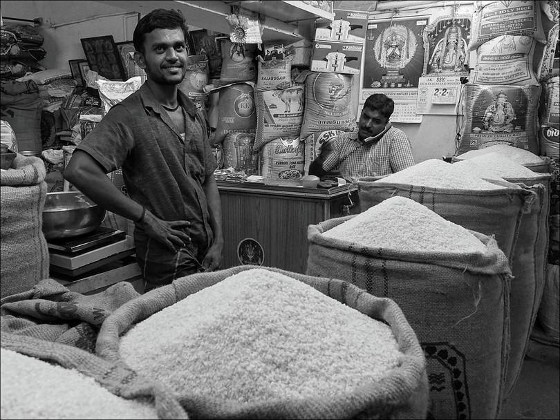
Figure C1.2 Rice traders displaying different varieties for consumption.
Romtomtom, Flickr, CC-BY 2.0.
If you go to any rice shop, you will find many different varieties of rice being sold. If you come from a paddy-growing area, you may even be aware that there are many different varieties of rice grown in your state. How can we understand this variation? Are different varieties really different? How can we identify and classify different varieties? Before you read further, spend some time thinking about these questions.
Exercise C1.2 Exploring rice varieties in your neighbourhood
Scientific processGo to a local shop and find out how many different varieties of rice are being sold there. How will you verify that these are different varieties? Would you trust the label on the package? Would you accept whatever the shopkeeper tells you? Are there independent ways you can make these identifications?
In this section, we will examine how different varieties of rice can be classified. We will first look at categorisation using physical and chemical properties and introduce a method known as hierarchical clustering. There are many properties that one can measure and we will explore whether all of them are necessary for categorisation. Finally, we will talk about phylogenetics, the use of DNA-based techniques for tracing the evolutionary history of rice varieties and for classifying them.
Directorate of Rice Development, Govt. of India
For more information on rice varieties, see these resources from the Indian Directorate of Rice Development:
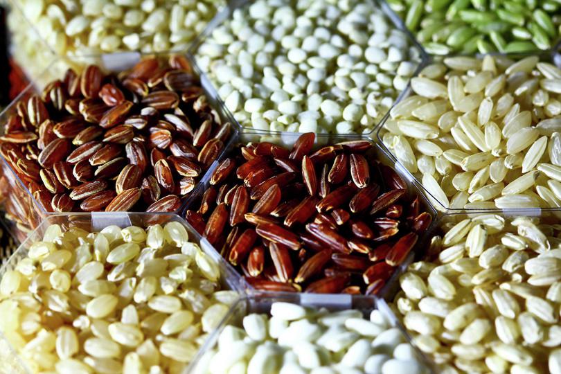
Identifying and categorising rice using physical and chemical characteristics
One way to tell different varieties of rice apart is to use physical and chemical characteristics such as colour, size, shape and aroma (Figure C1.3). Many scientists are interested in documenting unique rice varieties grown in their region. Such studies enable farmers to conserve local varieties and produce improved rice varieties through artificial selection. For example, they may breed rice varieties that have a desirable aroma or disease resistance.
Consider the research article written by Semwal, Pandey and Shariwal, in which they document 23 varieties from West Bengal.9 In this article, the authors provide information about the colour and aroma of these varieties. Imagine that friends returning from vacation bring you some rice grown in their native region. You want to find out whether it is one of the rice varieties documented by Semwal et al. How will you do that? You will probably look at a combination of characteristics. Does the rice have a similar colour as one of the documented varieties? Is the rice aromatic? Do rice grains have similar length and breadth? It is possible that these characteristics might allow you to roughly identify the rice that your friends gave you.
Researchers such as Semwal et al. use systematic methods to categorise different varieties. One variety may have different names in different regions.
Choosing variables
First consider the choice of variables. Read about how you can search for this information online. What variables have scientists used from the studies you found? Some variables are quantitative (they can be measured) and some are qualitative (they are described). You may be able to adopt a similar approach or adapt their approach for your purposes.
In a systematic study of six different rice varieties, Yadav, Khatkar and Yadav10 measured physical characteristics such as length and breadth of grains, chemical properties such as starch and amylose content, as well as how the varieties differ in terms of cooking (for example, how long it takes to cook them and how much the grains expand after cooking). These physical and chemical properties are quantitative variables, and the values are shown in Table C1.2.
| Cultivar | Thousand kernel weight (g) | Hardness (kg) | Amylose content (%) | Cooking time (min) | Elongation ratio | Width ratio |
| Jaya | 21.02 | 8.47 | 2.25 | 16.50 | 1.52 | 1.57 |
| HKR120 | 19.67 | 10.89 | 4.32 | 17.03 | 1.58 | 1.56 |
| P-44 | 17.13 | 11.34 | 5.97 | 17.40 | 1.66 | 1.46 |
| Sharbati | 14.82 | 11.19 | 7.10 | 17.53 | 1.75 | 1.39 |
| Bas-370 | 15.18 | 14.18 | 20.58 | 18.00 | 1.88 | 1.20 |
| HBC-19 | 17.03 | 15.77 | 22.21 | 18.30 | 1.89 | 1.14 |
Table C1.2 Physical, chemical and cooking properties of six rice varieties measured by Ritika Yadav and colleagues. See the entire set of measurements and explanations of the variables online.
Yadav, RB, Khatkar, BS and Yadav, BS, ‘Morphological, Physicochemical and Cooking Properties of Some Indian Rice (Oryza Sativa L.) Cultivars’, Journal of Agricultural Technology 3, no. 2 (2007): 203–210.
Association between variables
What can we do with the measurements shown in Table C1.2? Should we take all these variables into consideration? Firstly, group variables that are related in some manner. Choose different combinations of two variables and plot them against each other. Three examples are shown in Figure C1.4.
Identify which variables are associated with each other. Is the association positive, which means when one variable increases, the other variable also increases? Is the association negative, which means when one variable increases, the other decreases? Could there be a mechanism that causes one variable to affect the other? For example, based on Figure C1.4, is hardness responsible for a longer cooking time? Or, is there some underlying factor that influences both hardness and cooking time? In the next section, you will read more about the difference between association and causation. For the moment, we will restrict our concern to association.

Figure C1.4 Comparison of properties of six rice varieties measured by Yadav et al.
Adapted from Yadav, RB, Khatkar, BS and Yadav, BS, ‘Morphological, Physicochemical and Cooking Properties of Some Indian Rice (Oryza Sativa L.) Cultivars’, Journal of Agricultural Technology 3, no. 2 (2007): 203–210.
Using independent variables to classify rice
Exploring the association between different variables is a way of evaluating whether they are independent variables. If two variables are strongly related (knowing the value of one allows you to predict the value of the other one), then the variables are dependent and we can omit one of them. For example, in Figure C1.6, we can see that cooking time increases with hardness. We can use just one of these variables for comparison.
Suppose you have reduced your variables to only those that are independent. How can we use these variables for classifying rice varieties? Similar rice varieties should have similar values for all these variables. Rice varieties that are very different should differ in one or more of these variables. With this basic insight, we can use a method called hierarchical clustering to divide the rice varieties into different categories.
Hierarchical clustering technique
Clustering refers to any method by which individual objects (in this case rice varieties) are organised into groups based on some measure of distance or dissimilarity between them. Hierarchical clustering builds a hierarchy of clusters. Individual objects are grouped into clusters and then these clusters are further grouped into bigger ones. At the highest level, there is a single cluster containing all objects.
- dendrogram
- A tree diagram representing hierarchical relationships among objects or groups of objects. In biology, a dendrogram shows taxonomic relationships among species or groups of species.
The output of hierarchical clustering is depicted as a dendrogram (See Figure C1.5d). This provides information about which objects are similar to each other. It also shows the order in which different clusters are grouped into bigger ones. Clusters which get grouped before others contain objects that have more similarities than clusters that get grouped at a higher level.
Consider the process of hierarchical clustering using two independent variables: amylose content and thousand kernel weight (as shown in Figure C1.5d). We will use the distance between points as our measure of dissimilarity. (Ignore for the moment that the two variables have different units.)
- The points for varieties Bas-370 and HBC-19 are close to each other. They have similar values for the two variables and are grouped together in cluster 1. Similarly, HKR120 and Jaya are grouped into cluster 2 and the remaining two varieties are grouped into cluster 3. At this stage, all objects have been organised into clusters. See Figure C1.5a.
- Which two of the three clusters should be combined into a larger cluster first? Look at Figure C1.5b. The four lines shown in dark green are possible ways of connecting objects in clusters 1 and 2. The dissimilarity between these two clusters is the average of all four individual distances. Similarly, the four lines shown in pink connect objects in clusters 1 and 3. The dissimilarity between objects in clusters 2 and 3 (shown by light green lines) is the smallest.
- Using the dissimilarity index, cluster 2 and cluster 3 are combined first to form a larger cluster (cluster 4). See Figure C1.5c.
- Finally, cluster 1 and cluster 4 are combined and the distance between the objects is shown in blue in Figure C1.5c.
- The dendrogram shown in Figure C1.5d represents the clustering technique.

Figure C1.5 Procedure for hierarchical clustering based on properties of rice measured by Yadav et al.
Data from Yadav, RB, Khatkar, BS and Yadav, BS, ‘Morphological, Physicochemical and Cooking Properties of Some Indian Rice (Oryza Sativa L.) Cultivars’, Journal of Agricultural Technology 3, no. 2 (2007): 203–210.
a

b

c

d

e
Interpreting the dendrogram
Firstly, Bas-370 and HBC-19 are similar to each other. Secondly, they are different from the other four. Incidentally, Bas-370 and HBC-19 are basmati varieties and the other four are not. Therefore, the clustering process has indeed captured some information about the rice varieties.
Let us now recognise some subtleties related to interpreting dendrograms. Only vertical distances (indicated by d1, d2, d3) matter. The order in which the names of the varieties (called leaf nodes) appear and the horizontal distances do not matter. For instance, the two dendrograms shown in Figure C1.5d and Figure C1.5e convey the same information even though the labels at the bottom are in different order.
The dissimilarity between HBC-19 and Jaya is actually d3 even though the two varieties are indicated next to each other horizontally. Look at the vertical distance from the variety names to the point where clusters containing the two varieties are grouped. This grouping happens only at the very top. Similarly, the dissimilarity between HKR120 and P-44 is d2, which is higher than d1, which is the distance between P-44 and Sharbati.
Now that you understand the technique of hierarchical clustering, let us return to the example of rice varieties from West Bengal. We can apply hierarchical clustering to more than two variables. The basic procedure remains the same as used in the example we discussed in Figure C1.5. However, we would have to compute distances in more than two dimensions. Semwal et al. used four variables (kernel size, kernel breadth, awn length, kernel weight) to construct a dendrogram of 23 rice varieties (Figure C1.6).

Figure C1.6 Dendrogram of 23 rice varieties based on four quantitative parameters (kernel size, kernel breadth, awn length and kernel weight).
Adapted from Semwal, DP, Pandey, A, Bhandari, DC, Dhariwal, OP and Sharma, K, ‘Variability Study in Seed Morphology and Uses of Indigenous Rice Landraces (Oryza Sativa L.) Collected from West Bengal, India’, Australian Journal of Crop Science, 8, no. 3 (2014): 460–468. CC-BY-NC.
Extra reading Limitations of hierarchical clustering
Like any data analysis method, we should be careful with hierarchical clustering. Consider the dendrogram shown in Figure C1.5d. The two variables, amylose content and thousand kernel weight, have different units and should not be combined directly to compute a distance. Even if two variables have the same units, if one of them varies more than the other, it will have a greater impact on distance calculations.
Amylose concentration varies in value from 2 to 23, whereas kernel weight ranges from 14 to 22. Amylose concentration will have a greater influence on distance since it has a greater range of values.
In extreme circumstances, the variability of one variable can dominate all others. This is not ideal as the whole point of using multiple variables is to perform a more comprehensive comparison. Therefore, variables are often normalised before further analysis is performed.
Normalisation refers to changing the values so that all variables take approximately the same range of values or show the same variability. One way to normalise variables is to set the maximum and minimum observed values to 1 and 0 respectively and then scale all values in between proportionately. For example, a value halfway between the minimum and maximum would have a normalised value of 0.5. Panel A in the diagram below shows the dendrogram resulting from normalising amylose concentrations and thousand kernel weight before clustering. While the order of clustering has not changed, the distances have changed.

Effect of normalised variable choice on hierarchical clustering.
Data from Yadav, RB, Khatkar, BS and Yadav, BS, ‘Morphological, Physicochemical and Cooking Properties of Some Indian Rice (Oryza Sativa L.) Cultivars’, Journal of Agricultural Technology 3, no. 2 (2007): 203–210.
The variables chosen to perform clustering can affect the outcome. For example, the variables of cooking time and hardness produce the dendrogram shown in panel B. The dendrogram using cooking time alone is very similar (see panel C), since cooking time and hardness are related variables. Panel D shows the dendrogram produced by using all six variables (cooking time, hardness, elongation ratio, width ratio, amylose content, and thousand kernel weight).
While the choice of variables affects the dendrogram, there are some commonalities which are very informative. For example, Bas-370 and HBC-19 always group together and separately from the other four. Given that this result is consistent, we can confidently say that these two varieties are genuinely different from the other four.
Classification using genetic techniques
Physical and chemical characteristics provide a relatively simple means of classifying rice varieties. However, they present some challenges. Physical characteristics depend on the environment in which a particular variety is grown. Moreover, different individuals of the same variety may exhibit different physical characteristics. How can one address these challenges? Are there characteristics that are more stable and consistent?
Fortunately, the answer is yes. We can examine the DNA contained in these rice varieties. The growth environment does not affect the DNA sequence and will be very similar among different individuals of the same variety. Portions of the genome will differ in different varieties.
Genetic change and evolutionary history
Section C1.3 on evolution showed that modern rice varieties have descended from an ancestral wild species through domestication and breeding. Several genetic changes have been introduced during this process of domestication and breeding. Note that in the case of rice, genetic changes correspond to changes in DNA sequence.
Assume that we know what genetic changes have taken place in two different rice varieties and when in their evolutionary history these changes took place. What would we expect of two similar varieties? Most of the genetic changes would be shared and the changes that are not shared would have originated recently in their evolutionary history.
Less similar varieties will have fewer common genetic changes and the time at which their evolutionary histories diverged would be earlier. In other words, if we have access to the complete evolutionary history of different varieties, we can easily classify them based on how recently or how early these histories diverged from each other.
Unfortunately, evolutionary history is not available for most organisms, including varieties of rice. We have to reconstruct the evolutionary history based on data we can collect from varieties existing now.
Phylogenetics
- phylogenetics
- The study of evolutionary relationships between organisms.
The field of study known as phylogenetics aims to reconstruct the evolutionary history of groups of organisms. Before molecular biological techniques were developed, phylogenetics employed morphological and physiological characteristics like those used for hierarchical clustering. At present, phylogenetics predominantly uses molecular techniques based on the analysis of DNA sequences.
DNA analysis has many desirable properties, but it is more technically challenging and more expensive than morphological characteristics. DNA analysis requires specialised equipment and reagents, which require access to a laboratory. Also, molecular phylogenetic techniques are sophisticated and require some expertise to use properly. Fully appreciating these techniques and their nuances is beyond the scope of this text. However, we can try to build some intuition for these techniques through two examples.
Phylogenetic study of rice varieties
Upadhyay, Singh and Neeraja used DNA-based approaches to categorise rice varieties.11 They used a technique known as polymerase chain reaction (PCR) to amplify 20 different regions of the genome to produce DNA molecules of different lengths. Depending on the genetic sequence, each variety yields different PCR products.
The presence of the PCR product in a particular variety was scored as 1, whereas its absence was scored as 0. The researchers constructed a genetic signature consisting of 0s and 1s for each variety. Each PCR product is therefore a variable with a value of 0 or 1.
The researchers used the entire set of variables to construct a dendrogram using hierarchical clustering techniques (see Figure C1.7). How does this dendrogram indicate evolutionary history?
Varieties that are genetically similar would have diverged recently. These varieties would yield a similar set of PCR products. As a result, the distance computed between these varieties is likely to be small and they would cluster together before varieties that diverged earlier. Varieties in a cluster have a common history from the point they are clustered together until the top of the plot.
In Figure C1.7, the varieties Sarjoo 52 and Jayshree cluster at the very bottom. This indicates that they are genetically very similar to each other and diverged recently. In contrast, the varieties Sarjoo 52 and IR64 cluster near the top of the plot. They are genetically more distinct and diverged further back in time than Jayshree and Sarjoo 52.

Figure C1.7 Classification of 29 rice varieties using genetic and molecular biology techniques.
Adapted from Upadhyay, P, Singh, VK and Neeraja, CN, ‘Identification of Genotype Specific Alleles and Molecular Diversity Assessment of Popular Rice (Oryza Sativa L.) Varieties of India’, International Journal of Plant Breeding and Genetics 5, no. 2 (2011): 130–140.
Upadhyay et al. described the construction of a phylogeny of rice varieties with information about the presence or absence of particular genomic segments. With modern genetic tools, it is possible to obtain the entire genomic sequence of rice varieties and to compile a comprehensive list of genetic differences. This is, of course, a much richer set of genetic data and enables more sophisticated analysis of evolutionary history.
Extra reading Word ladders as an analogy for molecular phylogenetics
Before we explore an example of this kind, let us take a detour into the word game known as word ladder. The goal of the word ladder is to convert a given word into another one by changing one letter at a time. At each step, the new word should exist in an English dictionary. Panel A of the figure entitled ‘Word ladder’ shows how one can convert the word FOOT to COLD in three steps (with FOOD and FOLD as intermediates). To appreciate molecular phylogenetics, let us imagine a different variant of the word ladder. You have a set of words (COLD, BOLD, COOL, POOL). You are told that all words in this set are the final step in some word ladder game that all start from the same word. In the variant, the goal is to identify the common starting word and the sequence of letter substitutions that would give rise to all the words in the set. In the particular example, you can come up with at least two separate possibilities for the common starting word (FOOD and TOLL, in Panel B). With these two starting words, all the four words in the set can be reached after two substitutions. However, you can also come up with scenarios that either require more substitutions or an unequal number of substitutions for different words in the set (in Panel C).

Word ladder
- maximum parsimony
- An approach that assumes that the most likely method through which evolution has occurred is through the smallest number of steps required for a species to evolve.
We can now talk about how this variant of the word ladder game is similar to molecular phylogenetics. Firstly, we can only obtain DNA (or protein) sequences from varieties that are present today (the equivalent of the words shown in red). We are interested in inferring the evolutionary history of all these sequences, in other words, the sequence of genetic changes from a common ancestor that gave rise to all these sequences. This is similar to finding the common word from which all the words shown in red can be obtained. The word ladder variant illustrates some of the complexities of molecular phylogenetics. First of all, the sequence information is usually insufficient to determine the evolutionary history uniquely (the starting word could be FOOD or TOLL). Secondly, without additional criteria, one can potentially come up with a limitless set of scenarios all of which give rise to the same set of sequences (scenarios like Panel C).
You might be inclined to think that the scenarios shown in Panel B are better. One reason you might think so is that they require fewer substitutions than the scenarios shown in Panel C. In molecular phylogenetics, this line of reasoning is the basis of the criterion known as maximum parsimony. Is there any way to distinguish between the two scenarios shown in Panel B? With biological sequences, it is known that some changes are more likely to occur than others, and this may allow us to prefer one scenario over another. In the word ladder example, if it were the case that O → L substitutions were more likely than L → O, then it would be more likely for FOOD to be the starting word as opposed to TOLL.

Rooted and unrooted phylogenetic trees.
Let us now consider another complexity of molecular phylogenetics by examining the figure entitled ‘Rooted and unrooted phylogenetic trees’. In the two scenarios shown in Panels A and B, the total number of substitutions is the same. What is the difference between the two scenarios? In Panel A, all four words (COLD, BOLD, COOL, POOL) have started from FOOD and have been obtained by making two changes. In contrast, the way to interpret the scenario shown in Panel B is that all four words started from FOLD. Within the same time, COLD and BOLD underwent one change, whereas COOL and POOL had three changes, so changes have not taken place at the same rate throughout. You might be tempted to infer that the scenario in Panel A is better than the one in Panel B. You might justify this by noting that all the words shown in red have the same number of substitutions from the common starting word.
With biological sequences, a similar criterion is often used, known as the molecular clock hypothesis, which is that changes to molecular sequences occur at the same rate. The molecular clock hypothesis need not always hold and the number of character changes need not be equal along all branches (see Figure IV.8 from the evolution primer for an example). In the absence of additional criteria such as the molecular clock hypothesis, it may not be possible to find the starting point (and therefore the order in which changes occurred, that is, whether FOOD changed to FOLD or the other way around). In such cases, one often comes up with a plot like the one in Panel C. This plot shows how similar or different the four words shown in red are. This can be found by adding up the lengths of the lines joining two different words, for example, BOLD and POOL are four units apart, whereas BOLD and COLD are only two units apart. However, there is insufficient information to infer what the starting point is and therefore whether Panel A or Panel B is correct. In the context of molecular phylogenetics, plots similar to the one shown in Panel C represent an unrooted phylogeny (the root is the name given to the starting point).
Now that we have developed some intuition for molecular phylogenetics, let us grapple with another important aspect of the analogy between the word ladder and molecular phylogenetics. What is the biological equivalent of substituting letters in the word game? Mutations, of course. Point mutations, to be precise, or changes to DNA sequence that affect one or a few bases. Substitutions (where one DNA base gets replaced with another) are one kind of point mutation. Insertions/deletions (where one or more bases get added or deleted) represents another kind. So far, we have ignored the possibility of insertions/deletions. If bases are lost or gained, then sequences will no longer remain of the same length. This makes phylogenetic analysis much more difficult. How does one perform phylogenetics while taking insertion/deletions into account? We will again use the familiar world of words to develop some intuition.

Alignment can be used to account for insertions/deletions when performing phylogenetic analysis.
We have a set of six words (BOLD, COLD, COOL, FOOLS, FOLDS, POOL). We would like to infer the history of this set of words. A common approach to this problem is to make an alignment. The alignment process tries to match all the letters that are in common to all the sequences and introduces gaps (–) to account for deleted bases. All the aligned sequences are of the same length (if you count the gaps as well). In the example shown in the figure, all the alignments have six characters (with one or two gaps in each alignment). Using the alignment, it is possible to compute a distance between each pair of words. The distance shown in the figure is the minimum number of substitutions, insertions or deletions required to convert one word to another. (When working with biological sequences, just counting the number of mutations may be problematic. First of all, this treats both substitutions and insertions/deletions equally and that is not realistic.) For example, converting FOLDS to BOLD requires two changes: FOLDS → FOLD → BOLD, the first one is a deletion, the second is a substitution. Once we have a distance matrix, we can use methods similar to hierarchical clustering to group the sequences together and produce a dendrogram, which illustrates the phylogeny (the evolutionary history).
Dendrograms, phylograms and cladograms
- Dendrogram refers to any hierarchical or tree-like structure. In phylogenetics, they are referred to as phylogenetic trees.
- Phylograms, chronograms and cladograms are dendrograms produced through phylogenetic analysis. In a chronogram, the branch lengths represent evolutionary time. In a phylogram, the branch lengths are proportional to the number of changes in sequence. (Figure IV.8 in the evolution primer is a phylogram). A cladogram represents an evolutionary sequence without evolutionary time or number of changes.
McNally et al.’s phylogenetic study of rice varieties
To conclude the discussion of phylogenetics, we briefly look at an example of classification of rice varieties using genomic sequences. McNally et al. studied the DNA sequence of a large segment of the genome of 20 varieties of rice.12 They used sophisticated computational techniques to identify the genetic differences between these varieties and to produce a phylogeny (Figure C1.8). Their study identified as many as 160 000 genetic differences among the 20 varieties, whereas Upadhyay et al. studied 87 genetic differences.
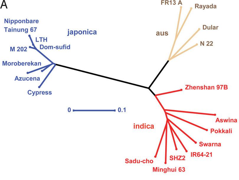
Figure C1.8 Phylogenetic tree constructed from genomic sequences of 20 rice varieties from McNally et al., 2009
McNally, KL et al., ‘Genomewide SNP Variation Reveals Relationships among Landraces and Modern Varieties of Rice’, Proceedings of the National Academy of Sciences 106, no. 30 (2009): 12273–12278, doi: 10.1073/pnas.0900992106. PNAS exclusive license to publish for non-commercial and educational use.
Figure C1.8 looks different from the dendrograms we have discussed so far. This is because it is an unrooted phylogeny (as explained in the extra reading on word ladders). The lengths of the various lines represent distances between different strains. We cannot identify the ancestral strain from which all of these varieties arose as there is no root. The authors were able to distinguish between japonica and indica varieties, as you would expect.
Since genomic sequence data is much richer than data on the presence or absence of genomic segments, the authors of this study were able to go beyond producing a phylogeny. The researchers were able to identify the portions of the genome in one variety that originated from a very different variety.
Identifying portions of the genome from different varieties allows scientists to uncover the breeding history of current varieties of rice. McNally et al. mention the example of Pokkali, a variety indigenous to India, which contains genomic portions from non-indica varieties. One of these genomic portions is associated with salt tolerance, an important trait for breeding. The authors suggest that early rice farmers in India might have cross-bred native varieties (those found in India) with exotic rice varieties (those from outside).
Naming and documenting varieties of rice
By now, you should appreciate how physical, chemical and genetic characteristics can be used to identify and categorise rice varieties. Why is it important to name and document rice varieties? Are there any benefits of doing so?
Naming allows information to be shared. What is the best way of growing a particular variety of rice? What are its useful or distinguishing characteristics? It would be very difficult to share knowledge about such questions without having a common set of names for referring to varieties. Another important reason to document our rice heritage is to protect indigenous knowledge and intellectual property from exploitation through ‘bio-piracy’.
Summary
In this section, we examined categorisation as a way of understanding biological diversity. In particular, we discussed how different varieties of rice can be classified using their physical and chemical properties as well as their DNA sequences. We illustrated a general procedure known as hierarchical clustering through which we can organise any set of objects into groups. Objects that are similar will be clustered first, and the order of clustering can be visualised through a dendrogram. For efficiency, it is better to use variables that are independent of each other. Such variables provide information that allows us to distinguish between similar objects.
We also developed an understanding of phylogenetics, the field of biology that seeks to reconstruct the evolutionary history of biological species (or individuals) using measurements performed on varieties that exist in the present. Modern genetic techniques are powerful scientific tools that allow us to characterise differences in DNA sequences on an unprecedented scale. Using such rich data sets of DNA variation, we can reconstruct the evolutionary history and categorise biological diversity.
C1.6 White rice and diabetes
Scientific process Quantitative skills
Rice is a staple food in many parts of India. Although, historically, millets (small seeded grasses) were consumed in greater quantities, rice has now generally displaced millet as the main source of carbohydrates. Have there been any consequences to this change in diet?
Figure C1.9 shows that the outermost layer of rice is a husk that protects the grain. Dehusking results in brown rice, which retains the bran layer. Further processing through milling and polishing removes the bran layer and yields white rice. White rice is only the rice kernel and germ layer.
White rice is a highly processed form of rice. What happens when we eat white rice, especially to blood sugar levels? It gives a quick burst of glucose in the blood stream. Brown rice on the other hand results in a slower release of glucose, allowing cells enough time to absorb the blood sugar (see Exercise C1.3).13 This is a very simplistic view of metabolism, as many other processes are taking place at the same time. But this description sets the stage for the next observation: the incidence of diabetes among Indians is extremely high.

Figure C1.9 Schematic of a rice grain.
The glycemic index (GI) is a value given to foods based on how slowly or quickly they increase blood glucose levels. Glucose is taken as a reference with a GI of 100. All others are measured relative to glucose. Complex carbohydrates present in fruits and vegetables typically have a GI of less than 50; simple carbohydrates found in white bread, polished white rice, cake and candy have a GI of more than 70. GI is also affected by what a particular food is eaten with. For example, white rice with higher GI can be eaten with daal (lentils) which has a lower GI, to get a more balanced GI.
Exercise C1.3 Comparing nutritional content of rice and millets
Quantitative skillsTable C1.3 compares Bapatla rice, a popular high-yielding variety of rice grown in Tamil Nadu and Kerala, to white rice and two millets.
- Compare the protein, fat and carbohydrate content of brown rice and white rice.
- Compare the protein, fat and carbohydrate content of both types of millets with brown rice and white rice respectively.
- Compare the glycemic index (GI) of millets and white rice. Which of them would result in a rapid increase in blood glucose when eaten?
Protein
(% g)Fat
(% g)Carbohydrates
(% g)Glycemic index Bapatla rice (brown rice 0% polish) 9 ± 0.1 2.3 ± 0.2 67 ± 0.3 57.6 ± 6.8 Bapatla rice (white rice 9.7% polish) 6.7 ± 0.1 0.5 ± 0.03 76.1 ± 0.5 79.6 ± 6.8 (Bajra) pearl millet 11.6 5 67.5 55 Foxtail millet 12.3 4.3 60.9 33 Table C1.3 Nutritional profiles of rice and millets along with glycemic values (% g represents macromolecules in 100 gram). Values vary with the type of cereal, its processing, individual metabolic rate and other food with which it is eaten.
Rice data obtained from Shobana, S, et al. ‘Even Minimal Polishing of an Indian Parboiled Brown Rice Variety Leads to Increased Glycemic Responses’. Asia Pacific Journal of Clinical Nutrition 26, no. 5 (2017): 829–836, doi: 10.6133/apjcn.112016.08.
Millet data obtained from Wahlang, B and Joshi, N, ‘Glycemic Index Lowering Effect of Different Edible Coatings in Foxtail Millet’, Journal of Nutritional Health & Food Engineering 8, no. 6 (2018): 404–408, doi: 10.15406/jnhfe.2018.08.00303.
Diabetes
Diabetes is a metabolic condition characterised by prolonged hyperglycaemia, or high blood sugar. Hyperglycaemia in diabetics occurs because the body is unable to use glucose effectively. In non-diabetics, the hormone insulin regulates how and when glucose enters the cells from the bloodstream. In diabetics, either not enough insulin is produced (type 1 diabetes), or the body is not able to use the insulin effectively (type 2 diabetes). Uncontrolled hyperglycaemia can lead to a wide variety of complications including kidney damage, retinal damage (leading to blindness), heart disease, and damage to feet and legs.
Figure C1.10a shows rice production across the globe, whereas Figure C1.10b shows the number of adults living with diabetes. China and India are the top producers of rice. India is second only to China in the incidence of diabetes. Long-term consumption of refined cereals is associated with a higher risk of type 2 diabetes and cardiovascular disease, particularly in Asian countries.14 15 16
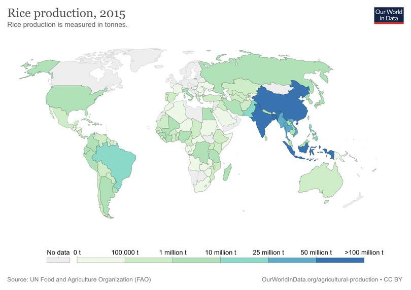
Figure C1.10a Map of rice production in the world.
Our World in Data, CC BY.

Figure C1.10b Incidence of diabetes globally.
Data from IDF Diabetes Atlas 7th edition.
Hu et al.16 shows that as white rice consumption increases, the risk of diabetes also increases, and this trend is similar for both Western and Asian populations (Figure C1.11).

Figure C1.11 Relationship between risk of type 2 diabetes and white rice consumption. Filled circles = Western populations; open circles = Asian populations. Size of the circle is proportional to the number of individuals tested.
Hu, EA, Pan, A, Malik, V and Sun, Q, ‘White Rice Consumption and Risk of Type 2 Diabetes: Meta-Analysis and Systematic Review’, BMJ 344 (2012): e1454, doi: 10.1136/bmj.e1454. CC BY-NC 2.0.
While the statistical analysis conducted to obtain Figure C1.11 is beyond the scope of this book, note that the relative risk (green line) increases steadily as the portion of white rice eaten per day increases.
Cause and correlation
Do these observations suggest that white rice causes diabetes? As an analogy, consider the wireless subscriber base in India. The number of people who subscribe to wireless services for their cell phone has increased substantially over the last two decades. Simultaneously, the number of people living with diabetes has increased. Consider Figure C1.12. Does it suggest that wireless subscriptions increase the prevalence of diabetes? The question may seem absurd but it is similar to the white rice question.

Figure C1.12 Number of adults living with diabetes in India versus wireless subscriber base in India from 2000 to 2015.
Data from Telecom Regulatory Authority of India, and Rhodes, EC, Gujral, UP and Narayan, KM, ‘Mysteries of Type 2 Diabetes: The Indian Elephant Meets the Chinese Dragon’, European Journal of Clinical Nutrition 71, no. 7 (2017): 805–811, doi: 10.1038/ejcn.2017.93.
This is the difference between cause and correlation. Both the risk of diabetes and wireless subscriptions are positively correlated with the consumption of white rice (which also has increased over the years). That is, when one variable changes, the other also appears to change with it. It would be incorrect to say, based on the data shown in Figure C1.11, that white rice causes diabetes.
The distinction between cause and correlation is very important. Let us try a few thought experiments to see if they can help establish a causal relationship.
A causal relationship is often very hard to establish, especially because there are often multiple interactions that lead to a disease state. In fact, there is no single known cause for diabetes, although many risk factors are involved.
Three important factors – diet, lifestyle and variants of certain genes – together affect susceptibility to diabetes, and have led to its global prevalence.15 For example, an unhealthy diet (a high carbohydrate, low fibre, high GI, high trans-fat diet), sedentary lifestyle (sitting for extended periods of time with no exercise), and a genetic predisposition lead to higher chances of diabetes.16 Many people who do not have any risk factors at all are diabetic. Therefore, although diabetes is widespread, a single cause has yet to be found. The distinction between cause and correlation is very important in any scientific study; too often, a correlation is confused with a causal relationship.
Summary
In this section, we looked at the relationship between rice consumption and type 2 diabetes. We saw that both the number of cell phone subscribers and white rice consumption are associated with type 2 diabetes. However, there is a distinction between correlation and causation. We saw that there is no single cause for diabetes, though there are several risk factors such as unhealthy diet, lack of exercise and genetic predisposition.
Establishing causality is a difficult task in most disciplines. Interpreting an association as indicating causality is a common mistake.
C1.7 Quiz
Question C1.1 Choose the correct answer(s)
Which of the following is involved in the production of white rice from freshly harvested rice?
- Milling is an important part of rice processing (see Figure C1.9).
- Read section C1.3 to learn about directional selection. This is an evolutionary phenomenon, not something involved in the processing of rice.
- Hierarchical clustering is a method for grouping objects into clusters and it has no role in rice processing. Read section C1.5 to know more about this technique.
- De-husking is an important part of rice processing (see Figure C1.9).
Question C1.2 Choose the correct answer(s)
Which of the following are negative consequences of the green revolution?
- Pesticides contaminate air, water and soil and affect plant and animal life.
- The green revolution emerged as a response to concerns that there would be widespread starvation due to population growth.
- Monoculture has led to loss of biodiversity. Any disease that can affect the varieties that are grown can spread over a wider area.
- Excessive use of fertilisers changes the nutrient balance in the soil and increases salt concentration.
Question C1.3 Choose the correct answer(s)
Indica and japonica varieties of rice have evolved from the ancestral wild grass Oryza rufipogon. Which of the following processes played an important role in this evolution?
- Artificial selection played an important role in the development of different rice varieties. Read section C1.3 for more information.
- Indica and japonica varieties were around long before the genome sequencing of rice plants became feasible.
- While the green revolution did change the varieties of rice that were grown, indica and japonica varieties were around long before the green revolution began.
- Indica and japonica varieties were around before the colonisation of India.
Question C1.4 Choose the correct answer(s)
Consider the measurements of two variables (A and B) shown in Table C1.4.
| Rice Variety | Variable A (observed value) | Variable B (observed value) |
|---|---|---|
| Variety 1 | 13 | 27 |
| Variety 2 | 63 | 91 |
| Variety 3 | 27 | 78 |
| Variety 4 | 43 | 127 |
| Variety 5 | 42 | 110 |
Table C1.4 Observed values of variables A and B.
One way to normalise the measurements is to use the following formula:
\[\begin{align*} \text{normalised value} &= \ \frac{(\text{observed value} - \text{minimum value})}{(\text{maximum value} - \text{minimum value})} \end{align*}\]This will convert the highest observed value to a normalised value of 1 and the lowest observed value to 0. Which of the following statements are correct?
- The minimum and maximum values of variable A are 13 and 63 respectively, and the observed value for Variety 4 is 43. Substitute these values in the formula.
- The minimum and maximum values of variable A are 13 and 63 respectively, and the observed value for Variety 3 is 27. Substitute these values in the formula.
- The order will be the same if you use observed values instead of normalised ones. You may have looked at variable A by mistake.
- The normalised value will be 1 for the highest observed value.
Question C1.5 Choose the correct answer(s)
Consider the measurements of variable A in five different varieties of rice.
| Rice variety | Variable A (observed value) |
|---|---|
| Variety 1 | 13 |
| Variety 2 | 63 |
| Variety 3 | 27 |
| Variety 4 | 43 |
| Variety 5 | 42 |
Table C1.5 Observed values of variable A.
If you perform hierarchical clustering using Variable A, which two varieties will cluster first?
- The first two varieties that will be clustered must have observed values closest to each other.
- The first two varieties that will be clustered must have observed values closest to each other. Read section C1.5 for more information.
- The first two varieties that will be clustered must have observed values closest to each other. Read section C1.5 for more information.
- The first two varieties that will be clustered must have observed values closest to each other. Read section C1.5 for more information.
Question C1.6 Choose the correct answer(s)
Which of the following are qualitative variables that can be used to characterise rice varieties?
- Length is a quantitative variable, which can be measured using a scale.
- Amylose content is quantitative and can be measured using chemical methods.
- Aroma is usually described in words and is qualitative.
- Grain colour is usually described in words and is qualitative. However, it is possible to quantify colour by carefully measuring wavelengths of light absorbed by the grain.
Question C1.7 Choose the correct answer(s)
The following image is taken from the Webcomic xkcd.
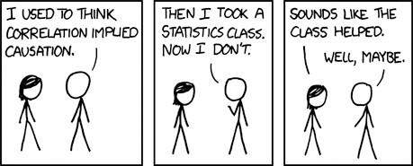
Cartoon correlation and causation.
Randall Munroe, xkcd, CC-BY-NC 2.5.
Which of the following best describes the point made by this comic?
- The cartoon definitely establishes a connection between attending the class and understanding the difference between correlation and causation.
- If these concepts were not taught in the class, the person on the right should have replied ‘no’ instead of ‘well, maybe’.
- Correlation and causation are not the same. Read section C1.6.
- If one factor is the cause of another one, then the two are likely to be associated. However, this is not the point being made by the cartoon.
Question C1.8 Choose the correct answer(s)
When a person eats equal quantities of two different varieties of cooked rice, the blood sugar level changes, as shown in the graph. One variety is white rice while the other is brown rice. The glycemic index of glucose is 100, and that of rice Variety 1 is 76.

Variation in blood sugar level when two different varieties of rice are eaten.
Which of the following statements are accurate?
- White rice has a higher glycemic index than brown rice.
- White rice has a higher glycemic index than brown rice. Variety 1 has a higher glycemic index.
- Variety 1 has a GI of 76. Variety 2 has a lower GI than Variety 1, therefore it has a lower GI than glucose.
- Glucose has a glycemic index of 100, and Variety 2 has a lower GI than Variety 1, which has a GI of 76.
C1.8 References
-
Ludden, D, An Agrarian History of South Asia, The New Cambridge History of India (Cambridge: Cambridge University Press, 1999), doi: 10.1017/CHOL9780521364249. ↩
-
Wikipedia, Malthusianism, accessed 18 February 2021. ↩
-
Thomas, G and De Tavernier, J, ‘Farmer-Suicide in India: Debating the Role of Biotechnology’, Life Sciences, Society and Policy 13, no. 1 (2017), doi: 10.1186/s40504-017-0052-z. ↩
-
Bridson, DM and Forman, L, The Herbarium Handbook (London: Royal Botanic Gardens, 1998). ↩
-
Penn State Extension, ‘Plant Identification: Preparing Samples and Using Keys’, (22 October 2007), accessed 1 March 2021. ↩
-
Honey, JN and Paxman, HM, ‘The Importance of Taxonomy in Biological Education at Advanced Level’, Journal of Biological Education 20, no. 2 (1986): 103–111, doi: 10.1080/00219266.1986.9654795. ↩
-
Khush, GS, ‘Origin, Dispersal, Cultivation and Variation of Rice’, Plant Molecular Biology 35, no. 1 (1997): 25–34, doi: 10.1023/A:1005810616885. ↩
-
Kovach, MJ, Sweeney, MT and McCouch, SR, ‘New Insights into the History of Rice Domestication’, Trends in Genetics 23, no. 11 (2007): 578–587, doi: 10.1016/j.tig.2007.08.012. ↩
-
Semwal, DP, Pandey, A and Shariwal, OP, ‘Variability Study in Seed Morphology and Uses of Indigenous Rice Landraces (Oryza Sativa L.) Collected from West Bengal, India’, Australian Journal of Crop Science 8, no. 3 (2014): 460–467. ↩ ↩2
-
Yadav, RB, Khatkar, BS and Yadav, BS, ‘Morphological, Physicochemical and Cooking Properties of Some Indian Rice (Oryza Sativa L.) Cultivars’, Journal of Agricultural Technology 3, no. 2 (2007): 203–210. ↩ ↩2
-
Upadhyay, P, Singh, VK and Neeraja, CN, ‘Identification of Genotype Specific Alleles and Molecular Diversity Assessment of Popular Rice (Oryza Sativa L.) Varieties of India’, International Journal of Plant Breeding and Genetics 5, no. 2 (2011): 130–140. ↩
-
McNally, KL et al., ‘Genomewide SNP Variation Reveals Relationships among Landraces and Modern Varieties of Rice’, Proceedings of the National Academy of Sciences 106, no. 30 (2009): 12273–12278, doi: 10.1073/pnas.0900992106. ↩
-
Shobana, S et al., ‘Even Minimal Polishing of an Indian Parboiled Brown Rice Variety Leads to Increased Glycemic Responses’, Asia Pacific Journal of Clinical Nutrition 26, no. 5 (2017): 829–836, doi: 10.6133/apjcn.112016.08. ↩
-
Radhika, G et al., ‘Refined Grain Consumption and the Metabolic Syndrome in Urban Asian Indians (Chennai Urban Rural Epidemiology Study 57)’, Metabolism: Clinical and Experimental 58, no. 5 (2009): 675–681, doi: 10.1016/j.metabol.2009.01.008. ↩
-
Hu, FB, ‘Globalization of Diabetes: The Role of Diet, Lifestyle, and Genes’, Diabetes Care 34, no. 6 (2011): 1249–1257, doi: 10.2337/dc11-0442. ↩ ↩2
-
Hu, EA, Pan, A, Malik, V and Sun, Q, ‘White Rice Consumption and Risk of Type 2 Diabetes: Meta-Analysis and Systematic Review’, BMJ 344 (15 March 2012), doi: 10.1136/bmj.e1454. ↩ ↩2 ↩3
