I Numbers and scales in biology
I.1 Introduction
Throughout this book, you will have to engage with numbers and data. If you had studied physics as a subject in school, you would have begun with units and dimensions. It is unlikely that you would have explored these topics in a biological context. You might even think that biology is descriptive and not quantitative.
Through this primer, we want to emphasise why numbers and scales are important in biology. We want you to develop an intuition for length (how big or small biological objects are) and time scales (how slow or fast biological processes are). We also want you to familiarise yourself with logarithms.
We will begin with a review of length and time scales. Then, we will introduce logarithms and why they are useful. We will conclude this primer by talking about comparison of scales and why this is insightful in biology.
I.2 Length and Time Scales in Biology
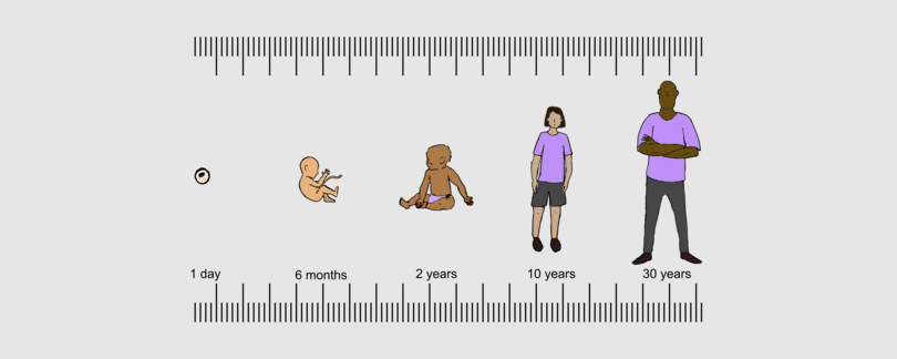
Biological phenomena span a wide range of length and time scales. What does this statement mean? How big is the nucleus in a typical animal cell? Over what distances do migratory birds travel? How quickly does the neuro-muscular system of a batsman need to react when facing a fast bowler in cricket? And how long does it take for a human baby to develop into an independent adult?
The numbers you come up with in response to these questions are vastly different. This illustrates that biological phenomena span a wide range of time and length scales. Moreover, if you expressed the numbers in the same units, you would have to deal with either very small or very big numbers. We will see below how logarithms make it convenient to deal with very small and very large numbers.
Length scales
Length scales characterise one dimension of the size of objects. One reason that biological objects span a wide range of length scales is the hierarchy of biological organisation (Figure I.1). Molecules are smaller than cells, cells are smaller than tissues, tissues smaller than organs, and so on.
The hierarchy of length does not account for all the size differences between biological structures. While the blue whale and the bumblebee bat (the world’s smallest bat) are both mammals, they are very far from being the same size!

Figure I.1 Hierarchy of life.
Can you name familiar length scales that are relevant to your everyday lives? Some examples that may come to your mind are your height, the distance to your school/college, the size of the room you sleep in, or the length of the lizard that crawls around your ceiling.
The relative size of objects becomes very important for our functioning. For example, the ceiling height should be greater than the tallest human in the house. Figure I.2 shows familiar length scales on the right, but what about length scales of very small living things and their components (the left side of Figure I.2)? Can we simply state that objects that are microscopic are all small, and ignore their relative sizes?
You might be surprised to know that human chromosome 1 (the largest human chromosome) is nearly 8.5 cm long. How can it fit inside the nucleus, which is much smaller in dimension? Understanding how the size of biological entities is regulated at the subcellular level is an active area of research. On a practical note, size is extremely important: abnormal or missing size regulation of microscopic entities, such as organelles, are often indicators of disease.

Figure I.2 Length scales.
Time scales
Just as each biological entity has a specific length scale, biological processes also take place at specific time scales. Some examples are illustrated below in Figure I.3. As with length scales, there are time scales that we encounter in everyday life and some that are beyond our limits of perception. Most reflexive actions (retracting your hand if you accidentally touch a hot object) occur over hundreds of milliseconds (one-tenth of a second). However, some cellular processes take place over a duration that is thousands of times faster than our reflex actions.

Figure I.3 Spatiotemporal scale for organising biological systems from large (for ecosystems) to sub-microscopic (for molecules). The time scale that is of relevance for these systems is shown on the right hand side.
Length and time scales are often related. The time scales relevant to phenomena occurring at small length scales are small (see lower part of Figure I.3). Secondly, most phenomena unfold both over space and time (see, for example, changes in land-use pattern described in section A3.1 and the epidemiology of malaria discussed in section B1.2). You will see the descriptive term ‘spatiotemporal’ in many texts (including this one) to refer to this aspect. Both location and duration are important things to study together in biological systems.
Why do length and time scales matter? Firstly, the length and time scales determine the techniques you will use to study the system. You will use a microscope to study bacterial cells, but not lions. Likewise, satellite imagery is useful for looking at forest cover over large regions, but is not useful for studying individual trees.
Secondly, it is sometimes possible to simplify an investigation by restricting ourselves to particular length and time scales. For example, we can study the behaviour of wild elephants by observing them over days, months or years without having to worry about how DNA is replicated in their cells.
I.3 Logarithms
The logarithm is a mathematical operation that is very useful for dealing with numbers that span a wide range. Before we formally define logarithms, we will first develop an intuitive picture for this concept. Then, we will look at some applications.
An intuitive picture of logarithms
Imagine that you have to count the number of trees in a garden. Let us say, the actual count is 27 and that you use tally marks (see Figure I.4) to count. Now, suppose that you have to convey this information to a friend. If you use tally marks to do so, you would have to draw 27 lines. On the other hand, if you use the decimal number system that is familiar to you, you only need to write 27, which is just two symbols (2 and 7). The difference would be even more stark if the count were larger (say 273). In this case, you would need 273 tally marks or just three decimal digits.

Figure I.4 Tally marks for counting 27 objects.
Both the number of tally marks and number of digits tell you the size of the count. A count requiring a greater number of digits is bigger. However, counts with the same number of digits can be vastly different. 100 is not the same as 999 even though both are three-digit numbers. In fact, 999 is almost a four-digit number.
As we will see in the section on the standard values of the base, the logarithm to base 10 will actually vary from 2 to 3 and not 3 to 4.
In order to distinguish between different three-digit numbers, we need a mathematical operation whose output increases smoothly from 3 to 4 as the count increases from 100 to 999. This is the intuition behind the logarithm.
The logarithm is a smoothing mathematical operation that takes a positive number as an input and produces another number as the output. The smoothness of the logarithm allows it to be defined for non-integer inputs too (for example, 100.5 instead of 100). For the moment, think of the logarithm as the number of digits required to represent the integer obtained by rounding off a given input number.
The ‘number of digits’ intuition does not work when the input is a positive number between 0 and 1. For such numbers, the decimal representation would be of the form 0.XXXX… . If we round such a number to the nearest integer, we will either get a 0 or a 1, both of which require one digit.
However, numbers in the interval 0–1 are not all equal. For example, 0.0003 is much smaller than 0.1. Observe, however, that the first non-zero digit after the decimal point occurs in the fourth position in 0.0003, whereas it occurs in the first position in 0.1. In this interval, the location of the first non-zero digit after the decimal point is an indication of how small the number is. The higher the position of this digit, the smaller the quantity.
If the input number is between 0 and 1, we can think of the logarithm as the negative of the position of the first non-zero digit after the decimal point. This would be −4 for 0.0003 and −1 for 0.1. Due to the negative sign, logarithms follow the natural order of their inputs (−4 is less than −1 just as 0.0003 is less than 0.1).
As with the number of digits, the position of the first non-zero digit is only a rough approximation. Both 0.0001 and 0.000 999 9 have the first non-zero digit at the fourth position. But, 0.000 999 9 is approximately 0.001 and so the logarithm should vary smoothly from −4 to −3 as its input changes from 0.0001 to 0.000 999.
Formal definition and properties
Mathematically, the logarithm is the inverse operation of exponentiation. Let us unpack this statement before we present the formal definition. First, we will look at more familiar examples of inverse operations. Then, we will revisit what exponentiation means. Finally, we will define the logarithm.
We know that addition and subtraction are opposites of each other. They are inverse operations. What does that mean? We know that \(5 + 3 = 8\). If we wanted to find the number which satisfies \(5 + \text{?} = 8\), the answer would be \(8 - 5 = 3\).
Subtraction and addition have opposite outcomes. In fact, if we add and subtract the same number, there is no change (for example, \((8 + 3) - 3 = (8 - 3) + 3 = 8\)). Multiplication and division are also examples of inverse operations. We know that \(5 \times 3 = 15\). We would solve the problem \(5 \times \text{?} = 15\) by carrying out the operation \(15 \div 5 = 3\).
Now that we understand what inverse operations mean, let us recap the definition of exponentiation. Exponentiation, in the simplest case, is equivalent to repeated multiplication. For example, we know that \(2 \times 2 \times 2 \times 2 = 16\). We can represent the same information as \(2^{4} = 16\), which we read as ‘two raised to the power of four is equal to 16’.
The operation of raising to a power is called exponentiation. The number \(2\) in \(2^{4}\) is called the base and the number \(4\) is the power or the exponent. Exponentiation can be thought of as repeated multiplication when the exponent is a positive integer.
It is possible to extend the concept of exponentiation to non-integral and negative numbers. For example, raising a number to a power of \(0.5\) is the same as taking the square root (\(4^{0.5} = \sqrt{4} = 2\)).
Let us now revisit the statement that the logarithm is the inverse operation of exponentiation. If we wish to solve \(2^\text{?} = 16\), we know the answer is \(4\). We refer to \(4\) as the logarithm of \(16\) to the base \(2\) and we represent this as \(\log_{2}16 = 4\). In other words, the logarithm is the power to which a base should be raised to obtain a given number.
We can now formally define the logarithm. The logarithm of a number \(x\) to base \(b\), which is denoted by \(\log_{b}x\) is the power that \(b\) has to be raised to in order to get a value of \(x\). In other words, \(\log_{b}x\) equals \(y\) if (and only if) \(b^{y} = x\). This definition is valid when the number \(x\) is positive. We will also assume that the base \(b\) is greater than one. Some examples of logarithms are shown below:
The formal definition holds even if \(b\) is between 0 and 1. However, the intuitive picture presented at the beginning of this primer will not be accurate. In practice, the values of \(b\) that are commonly used are greater than 1.
- \(\log_{10}1000 = 3\) because \(10^{3} = 10 \times 10 \times 10 = 1000\)
- \(\log_{4}2 = 0.5\) because \(4^{0.5} = \sqrt{4} = 2\).
- \(\log_{3}81 = 4\) because \(3^{4} = 3 \times 3 \times 3 \times 3 = 81\).
For completeness, we list some of the properties of logarithms below. In the properties, the bases \(a\) and \(b\) are positive numbers not equal to 1, the numbers \(x\) and \(y\) are any positive numbers and the number \(z\) is any real number (positive, negative or zero).
- \(\log_{b}xy = \log_{b}x + \log_{b}y\). For example,
\(3 = \log_{10}10^{3} = \log_{10}1000 = \log_{10}(100 \times 10) = \log_{10}100 + \log_{10}10 = 2 + 1\). - \(\log_{b}x/y = \log_{b}x - \log_{b}y\). For example,
\(2 = \log_{10}10^{2} = \log_{10}100 = \log_{10}(1000 \div 10) = \log_{10}1000 - \log_{10}10 = 3 - 1\). - \(\log_{b}x^{z} = z \log_{b}x\). For example,
\(3 = \log_{10}10^{3} = 3 \times \log_{10}10 = 3 \times 1\). - \(\log_{b}1 = 0\).
- \(\log_{a}x = \frac{(\log_{b}x)}{(\log_{b}a)}\). For example,
\(2 = \log_{4}16 = \frac{(\log_{2}16)}{(\log_{2}4)} = \frac{4}{2}\)
While you can read this book without being familiar with these properties, you will need to know how to read logarithmic scales (described below).
Standard values of the base
In the previous section, we saw the definition of \(\log_{b}x\). While the definition allows for any positive value of \(b\) (other than 1), there are three values of \(b\) that are most frequently used. These three values are described next and some representative values of logarithms to these bases are shown in the table below.
- The common logarithm uses 10 as the base \((b = 10)\). This corresponds to the intuitive picture described at the beginning of this section. As we are used to the decimal system, it is much easier for us to make sense of the common logarithm. If the common logarithm of a number is between 3 and 4, we know that the closest integer to the number has four digits.
- The natural logarithm uses the irrational number \(e \approx 2.718\) as the base. The natural logarithm of \(x\) is denoted by \(\log_{e}x\) or \(\ln x\). You might wonder why a strange number such as \(e\) is used as the base. The answer to this is technical in nature. We will just mention that \(e\) is a very convenient base for calculus. You may refer to a more elaborate explanation.
- Apart from \(10\) and \(e\), another base that is often used is \(2\). In biology, there are several contexts where powers of \(2\) are seen. Consider a cell that divides by mitosis to give rise to two daughter cells. If both daughter cells again undergo mitosis, we will get \(2 \times 2 = 2^{2} = 4\) cells. In general, starting from a single cell, we will get \(2^{n}\) cells after \(n\) mitotic divisions. Suppose we wish to know the number of divisions required to get 1000 daughter cells. We will need to solve \(2^{?} = 1000\). The answer would be \(\log_{2}1000 \approx 10 (2^{10} = 1024)\).
The values of logarithms to all three bases are proportional to each other and it is easy to convert between the three bases using the following formulas:
- \(\ln x = \ln 10 \times \log_{10} x \approx 2.303 \times \log_{10}x\).
- \(\log_{2} x \approx \log_{2}10 \times \log_{10} x \approx 3.322 \times \log_{10}x\).
- \(\log_{2} x \approx \log_{2} e \times \ln x \approx 1.443 \times \ln x\).
| \(x\) | \(\log_{10}x\) | \(\ln x\) | \(\log_{2} x\) |
|---|---|---|---|
| 0.0003 | −3.523 | −8.112 | −11.703 |
| 0.1 | −1.000 | −2.303 | −3.322 |
| 1 | 0.000 | 0.000 | 0.000 |
| 10 | 1.000 | 2.303 | 3.322 |
| 27 | 1.431 | 3.296 | 4.755 |
| 99 | 1.996 | 4.595 | 6.629 |
| 273 | 2.436 | 5.609 | 8.093 |
| 1000 | 3.000 | 6.908 | 9.966 |
Table I.1 Values of logarithms.
Applications of logarithms
Historically, one of the first applications of logarithms was to simplify calculations which had to be done manually. Today, all of us have access to a calculator (your mobile phone probably comes with a calculator app) and this application is less important. We will therefore look at how logarithms allow us to work with numbers that span several orders of magnitude and how they enable us to visualise certain kinds of relationships between variables.
Logarithmic scales
In biology, we encounter phenomena at vastly different scales (refer to Section I.2). Therefore, we often have to work with very small or very large numbers. For example, the length of a typical bacterial cell is around 0.000 001 metres. The diploid human genome, on the other hand, consists of around 6 000 000 000 basepairs of DNA. Working with such small or large numbers is cumbersome and error prone (it is easy to miss a zero!).
To avoid errors, we can either use units (1 µm for 0.000 001 metres and 6 Gbp for 6 000 000 000 basepairs; the prefixes µ and G represent \(10^{- 6}\) and \(10^{9}\) respectively) or use scientific notation (\(10^{- 6}\) m for 0.000 001 metres and \(6 \times 10^{9}\) basepairs for 6 000 000 000 basepairs).
Units and scientific notation may present difficulties if quantities vary over orders of magnitude. Consider the hydrogen ion concentration in your stomach and your blood. In your stomach, this may be as high as 0.03 M (moles per litre), whereas in your blood it would typically be around 0.000 000 04 M. We can represent these quantities as \(3 \times 10^{- 2}\) M and \(4 \times 10^{- 8}\) M respectively, but we will need to pay close attention to the exponents (−2 and −8).
Taking logarithms of these quantities will allow us to work with more convenient numbers. In fact, if we take logarithms to base 10 and multiply this by −1, we will get the familiar quantity known as pH. The pH of the stomach would be \(- \log_{10}0.03 \approx 1.5\) and your blood would have a pH of \(- \log_{10}0.000 000 04 \approx 7.4\). Would you agree that 1.5 and 7.4 are easier numbers to work with (assuming you are now familiar with logarithms)?
The pH is an example of a logarithmic scale. It illustrates one very useful property of logarithms, that of compressing numbers spanning orders of magnitude to a more convenient range. This property is often useful in plotting.
Consider the eight numbers shown in the first column of Table I.1. If we were to plot them on a standard number line, we would not be able to distinguish all eight points (see the top panel of Figure I.5). The values 0.0003, 0.1 and 1 overlap each other and we can’t tell them apart.
We can address this issue by plotting the logarithms of these quantities (see middle panel), that is, by using a logarithmic scale instead of a standard or linear scale. In order to ensure that the log scale is easy to read, we indicate the original values of the quantities (and not their logarithms). As can be seen from the figure below, all eight points are visible. In effect, we have compressed values spanning a large range into a smaller range.

Figure I.5 Reading log scales.
Typically, when a log scale is used, the location of powers of 10 are shown (see bottom left panel). Observe that powers of 10 (\(10^{2}\), \(10^{3}\), \(10^{4}\)) are clearly shown. Between consecutive powers of 10, you will notice 8 minor tickmarks, which are not equally spaced. What values do these represent?
To answer this question, consider the interval between \(10^{2}\) and \(10^{3}\). The first minor tickmark in this interval corresponds to a value of \(2 \times 10^{2}\). The next minor tickmark corresponds to \(3 \times 10^{2}\) and so on. If a value falls between the fourth and fifth minor tickmark (for example), then it is between \(5 \times 10^{2}\) and \(6 \times 10^{2}\). If there were a ninth minor tickmark, it would correspond to a value of \(10 \times 10^{2} = 10^{3}\), which is the next power of 10.
Sometimes, indicating minor tickmarks makes the scale very cluttered and these are omitted for clarity. There are also situations when the values that are shown are not powers of 10. How can one read such scales?
Assume that values \(a\) and \(b\) are indicated (refer to the bottom right panel) and we know that the scale is logarithmic. The value corresponding to the midpoint of this interval is \(\sqrt{ab}\).
For illustration, if \(a = 20\), \(b = 200\), then the point shown in blue corresponds to a value of \(y = \sqrt{ab} = \sqrt{20 \times 200} \approx 63.25\). Often, knowing the midpoint is sufficient to get a rough estimate of any point that is shown. To get a better estimate, we can repeat this procedure. For example, the point shown in green is exactly halfway between the midpoint and \(b\). Its value would be \(\sqrt{yb} = \sqrt{63.25 \times 200} \approx 112.5\).
One important thing to note about log scales is that we cannot plot zero on such a scale. This does create problems in some situations as zero is a value that we would like to show. Sometimes, this issue is addressed by artificially adding a small, positive number to the zero values.
Semilog and log-log plots
We often try to investigate the relationship between two variables by plotting one against the other. The first thing you might try would be to plot both variables using standard or linear scales. However, there are situations when using a log scale would be more informative. When one axis is linear and the other is logarithmic, we get a semilog plot. If both axes use a logarithmic scale, we obtain a log-log plot. We will now see why semilog and log-log plots are useful.
Consider the cell division example used earlier. At time 0, there is one cell. After 30 minutes, this cell divides to give rise to two daughter cells. After 30 more minutes (one hour from the beginning), these two cells will divide to give rise to four cells in total. Thereafter, every 30 minutes, the number of cells will double.
Cell division is an example of exponential growth. If we plot the number of cells against time using linear scales, we will get a curve similar to the one shown in Figure I.6a. On the other hand, if we use a log scale for the number of cells, we will get a semilog plot that is a straight line (see Figure I.6b). In fact, it is possible to estimate the generation time (time taken for a cell to divide) from the slope of the straight line in the semilog plot.
Exponential processes are quite common in biology and semilog plots can be used to identify an exponential relationship between two variables.

Figure I.6 Growth in number of cells shown on linear scales (A) and semi-log plots (B).
To conclude we examine an example of a log-log plot. Sometimes, two variables are related by what is known as a power law, that is, one variable is proportional to a fixed power of another variable.
The area of a circle is proportional to the square of its radius \((\text{Area} = \pi r^{2})\). By plotting area against radius using linear scales, we will get the curve shown Figure I.7a. A log-log plot is more insightful. If we use log scales for both axes, we will get a straight line as in Figure I.7b. Moreover the slope of the line is equal to the power (2 in this case). We will discuss a biological application of the log-log plot in the next section.

Figure I.7 Relationship between area and radius of a circle shown on linear scales (A) and a log-log plot (B).
Estimation and comparison of scales
Estimating values and comparing scales of different entities often reveal important insights into biological systems. Consider the example of human chromosome 1. We mentioned earlier that the human chromosome 1 is nearly 8.5 cm long. How did we get this estimate?
Based on the structure of DNA, we know that every base pair contributes 0.34 nm in length. There are roughly 249 million \((2.49 \times 10^{8})\) basepairs in chromosome 1. Multiplying 249 million by 0.34, we estimate the length of the chromosome to be approximately \(8.5 \times 10^{7}\) nm or 8.5 cm.
Take another example of estimation. What is the volume of a person weighing 50 kg? We know that most of our body weight is contributed by water, which has a density of 1 kg per litre. Therefore, the volume of the person would be estimated to be 50 litres.
Comparing values
Apart from estimation, comparison is also very informative. Imagine that we have two cells whose shapes are approximately spherical. Suppose that cell A has a radius of 10 µm, and cell B a radius of 100 µm. The radius for cell B is 10 times greater than cell A, but how does this influence the ability of the cell to exchange material with its environment?
The surface area (SA) of the cell may be a more appropriate and useful measure since exchange takes place at the surface of the cell. If we compute surface area, we get
- Cell A: \(r = 10 \text{ µm, SA} = 4 \pi r^{2} = 1200 \text{ µm}^{2}\)
- Cell B: \(r = 100 \text{ µm, SA} = 4 \pi r^{2} =120 000 \text{ µm}^{2}\)
From this simple calculation, we see that the surface area has increased 100 times when the radius increases only 10 times. This example shows us that not only is it important for us to compare scales, we should also consider the most appropriate measure to address the question at hand.
I.4 Allometry
Allometry is the study of relationships between the scales of different biological processes/entities in the same system. Take the example of the development of the human brain from birth to adulthood. The brain grows, but does it grow at the same rate as the rest of the body?
Measurements have shown that the brain stops growing by about age six. So, while the body continues to grow, the head size becomes proportionally smaller. The heart on the other hand, continues to grow at nearly the same rate as the body; that is, heart size scales linearly with body size.
Figure I.8 shows the relationship between the sizes of heart, brain and body in a log-log plot (natural logarithms are taken for both axes). The linear relationship appears as a straight line (it is a power law), whereas the relationship between brain size and body size reaches a fixed level once the logarithm of body size exceeds 9.5 (this corresponds to \(e^{9.5} \approx\) 13 000 g = 13 kg).
Such relationships often indicate an underlying mechanism. One possibility that explains the allometric relation of body size and heart size is that as the body grows, the amount of oxygen that has to be delivered via blood circulation may also increase proportionately.

Figure I.8 Body proportions at different ages.
Adapted from Shingleton, A, ‘Allometry: The Study of Biological Scaling’, Nature Education Knowledge 3, no. 10 (2010): 45–55.
Allometric scaling can be measured across species too – these relationships may provide ecological and evolutionary insight. The most famous (and still not fully understood) such relationship is the scaling between metabolic rate and body size, also known as Kleiber’s law. Overall metabolic rate (the rate at which animals use energy) scales as body weight raised to the power of 0.75. This relationship, which is a power law, can be visualised on a log-log plot, as shown in Figure I.9.

Figure I.9 Graph illustrating Kleiber’s law, or the relationship between metabolic rate and body size in animals.
This relationship hints at a possibility that a universal mechanism has persisted through evolution that regulates metabolic rate based on body size. Allometry is just one way in which studying how organisms behave over various spatiotemporal scales gives us insight into life.
We hope this primer allows you to appreciate how understanding scales deepens our sense of biology.
